Saturday, May 7, 2011

Data Validation List based on another data validation list

Have you ever thought how simple life could be if you could make your spreadsheets act more like a form without going through the trouble of creating one?  In today's example you can create a list of values in one field where another list is populated based on what the user selects!
Sub list2()
    With Cells(1, 2).Validation
            .Delete
        If Cells(1, 1) = "one" Then
            .Add Type:=xlValidateList, Formula1:="A, B, C"
            ElseIf Cells(1, 1) = "two" Then
                .Add Type:=xlValidateList, Formula1:="D, E, F"
            ElseIf Cells(1, 1) = "three" Then
                .Add Type:=xlValidateList, Formula1:="G, H, I"
        End If
    End With
End Sub
The above example will only refresh when the macro is run.  If you want this to run as soon as a value is chosen you may want to set this into the worksheet where an event will trigger it to run.

Thursday, March 3, 2011

Printing Multiple Sheets with VBA

Printing Multiple Sheets

Unhiding Multiple Worksheets

Most people who use Excel know that you can hide one or more sheets in Excel. Thanks to thesimplemachine.com we now have a short code for unhiding these sheets all at once rather than one at a time. Take a look!

Unhiding Multiple Sheets with VBA

Tuesday, March 1, 2011

Edit Multiple Selections in Excel Drop Down Lists

Microsoft has come up with an amazing array of features in Excel. One such feature is the drop down list which creates the ability for the user to provide feedback that drives other parts of the workbook. Gathering feedback from your audience not only allows your them to change scenarios as they see fit but it prevents you from recreating reports for each scenario.

As with any feature there are limitations. This is where the beauty of VBA comes into play! In yesterday's blog post from Contextures.com we are shown how you can handle problems with editing drop down lists:

Contextures Blog » Edit Multiple Selections in Excel Drop Down Lists

Thursday, February 24, 2011

John Walkenbach on Excel

To learn more about Excel, take a look at the selection of books now available from:

Mr Spreadsheet

Creating arrays using VBA

Now with an understanding of the power of arrays we can build upon this using VBA.  Here is a very thorough overview of arrays from a highly respected source:


Please visit our sponsors to the right for more resources available on Excel & VBA today!

Thursday, February 10, 2011

Valentines Day Excel Workbook VBA

Admittedly, this could be made into so much more of an elaborate greeting but then perhaps flowers or chocolates would be more suitable.  

This short script, when placed within the 'This Workbook' section in the project section in your VB browser, will activate any time a change is made to that workbook (i.e. selecting a cell).

Private Sub Worksheet_SelectionChange(ByVal Target As Range)
    x = MsgBox("Will you be my valentine?", vbYesNo, "Valentine Greeting")
    If x = 6 Then
        MsgBox "I am yours"
    Else
        MsgBox "Happy Valentines Day!"
    End If
End Sub

As you can see, a pop-up window will appear with the question "Will you be my valentine?"  If the user selects yes you see a new pop-up window with "I am yours".  If no is selected they will only see "Happy Valentines Day!".  Surprise the Excel geek in your life with a workbook today and a custom message of your choosing and have a happy valentine's day!

Monday, February 7, 2011

Highlight fields in vba rather than conditional formatting

Ever wanted to quickly highlight cells where the values are not found in another list?  Here is an example of how VBA can accomplish just that!


Notice that there is an error handling used 'On Error Resume Next'?  If you run this macro without it you will have problems but this statement allows the script to continue on even though the error exists!

Tuesday, February 1, 2011

Time my macro

Want a quick way to time your macro or demonstrate to your user how fast your macro runs?  Here is a quick code that will pop up a message box displaying the time it took!


Sub Time()
Dim Start As Long, Ending As Long, Time As Long
    Start = Timer()
        'insert macro here
    Ending = Timer()
    Time = Ending - Start
    MsgBox "Time lapsed: " & Format(Time / 60, "###.00") & " minutes or " & Time & " seconds"
End Sub

Excel Array Formula Series #8: FREQUENCY function

Saturday, January 29, 2011

User-Defined Function Argument Descriptions In Excel 2010

One of my favorite features in Excel is the user-defined function.  It can simplify an otherwise complicated function and allow you to personalize its labeling.


Spreadsheetpage.com has provided a great example of this in the following post.


Learn even more tips and tricks with John Walkenbach's book 'Favorite Excel Tips & Tricks' available now at Amazon.com!

Excel Array Formula Series #5: SUM 3 Largest Values

Monday, January 24, 2011

Drawing in Microsoft Excel

Why even bother declaring variables?

It may seem a bit of a hassle to declare a variable when you could just as easily reference that value (or cell containing that value) directly, right?

While there is nothing that says you cannot, you may find that as your code increases in length, it becomes ever more difficult to recall what value was in cell B1 or D4.  By creating a variable you can now add a name to it such as MyValue and you will find it far easier to follow and edit your code now (and especially down the road).

Whenever you use a value more than once without declaring it as a variable you are forcing Excel to look up that value over and over and over again.  Obviously, this takes time.  The more loops there are?  The more that time ads up.  Variables remain in the computer's memory for use whenever you need it!

Here is a great article on the many variable types available and further background on this topic!

Saturday, January 22, 2011

Converting values into English words

Ozgrid has published a neat trick on making Excel convert numbers into actual English words!  This could be quite handy for inserting into word documents or just to show off to your co-workers!

Friday, January 21, 2011

Excel Everest | The Math After the Party

Excel Everest | The Math After the Party

Needle in a haystack - Finding your formulas!

Have you ever found yourself faced with a huge table of data with some cells that contain formulas while others don't?  It can be like finding a needle in a haystack!  MrExcel has come up with a brilliant solution to this by enabling highlighting of formula cells!  Click on the link to the CFO.com article published by MrExcel for more:


Wednesday, January 19, 2011

Scroll Bars - Negatives & Decimals

Ever wish you could choose a different increment than a positive whole number?  With VBA you can accomplish both and far more.

In http://automatenow.blogspot.com/2011/01/scroll-bars-financial-modelling.html I introduced how scrolling bars were able to affect a graph in real time by linking that scroll bar to a cell and allowing the chart and corresponding graph to update based on the values.  The limitation is that you can only scroll from 0 - 30,000.

One way you can work around these limitations is by using VBA to create a value in one (or more) cells outside of the linked as shown here:

Although the value in cell A1 still changes by increments of 1 cell A2 can now be affected by any change in the very same scroll bar.  This is done by using the change method to the object scrollbar1.

Now, with the code above, any change in the scroll bar will launch the script to update cells A2 with the formula defined in that script with cell A1 - 50 * 0.25.  Move the scroll bar to 50 and the value in A2 becomes your new zero.  Move it to the left and you will see it progress down by 0.25 increments in the negative direction!

You can clean this worksheet up by dragging the scroll bar to cover up your linked cell (A1) to allow your user to only see the resulting -1.75 when the scroll bar value is actually 43.  Imagine now how easy it is to have several cells to apply complex formulas, functions or even text results driven by this scroll bar...

Friday, January 14, 2011

Wrapping text within a cell in Excel using VBA


The most simplest way to make a cell word wrap is to right click and format the cell alignment to wrap text.  This makes the text begin on the next line within that cell when it reaches the right cell wall.  You increase the size of the cell and more text appears on the first line with less on the next.


There may, from time to time, be a case where you need to begin a new line regardless of the size of that cell.  VB needs to see a carriage return in order to accomplish this.  A carriage return is represented by Chr(10) and may be inserted into the cell directly as follows:


ActiveCell.FormulaR1C1 = "ABCD" & Chr(10) & "EFGH"


Of course, you may want to incorporate this several times based on a specific length.  Here is one way this might be accomplished:


Sub AddCarriageReturns()
'
' Macro created 1/13/2011 by Steve Wynne
'
Dim CarriageInsert
Dim FullString As String
Dim I As Integer
'
I = Len(ActiveCell)
Do Until I = 5
    I = I - 5
    CarriageInsert = Mid(ActiveCell, I, 5)
    FullString = CarriageInsert & Chr(10) & FullString
Loop
    ActiveCell = FullString
End Sub


Try to nest this within a for/next or loop statement and it can be applied to an entire range of cells!

Wednesday, January 12, 2011

Win an Xbox & Kinect Package

For more go to the Excel contest tab on the Excel Group in Facebook

Calculations that slow you down

When you are working in a workbook you may find yourself frustrated by how slow it is performing.  Often the computer is the first to receive the blame but here are some areas to consider before throwing your pc out the window.

First, if you have a lot of formulas, ask yourself do I need them to constantly refreshing?  If the answer is no then try switching your calculation options to manual.  When you are done with all your set-up you can switch back to automatic or even hit F9 whenever you are ready to see your results.  

If the values provided by your formulas are all you need, and the values used in the calculations are no longer changing, try to copy| paste special then selecting values.

Using VBA you can use set the cell equal to the value of a given formula or function as follows:
  • Cells(1, 2) = Application.VLookup(Cells(1, 1), Range(Columns(4), Columns(5)), 2, False)
Notice how I reference the cells with numbers rather than letters? The first is the row reference and the second a column reference (opposite from the A1 you may be accustomed to).  These numbers can now be substituted by variables which is very handy when nesting formulas within loops or if/then statements.  

To learn more about the full range of formulas and functions available in Excel 2007:

Monday, January 10, 2011

Scroll Bars - Financial Modelling

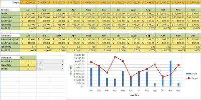
What do you do when you are given a set of targets to meet with a forecast that is not quite meeting them?  You may have several variables involved and you need to find what affect each change has to your model.  As they say, a picture is worth a thousand words, and when dealing with data it could be no further from the truth.

Enter the scroll bars pared with charting (click on image for full view):

Did you notice how the chart to the lower right is impacted by the change in variables?

For the user, you simply one or more of the scroll bars up/down to increase or reduce these input values to see (in real time) the impact within the chart to the lower right.  To create these scroll bars, you need to follow these 5 simple steps:
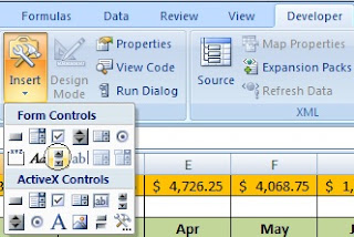
  1. From the developer ribbon select insert then choose the following:
  2. From the location you wish to locate this control click and drag to the size you wish this to be.
  3. Right click and select format control.
  4. From the control tab you can set your minimum and maximum values for this control and by what increment each click will change it.
  5. In cell link choose the destination for the value present in the scroll bar.

For a more about modeling with Excel 2007
 

Sunday, January 9, 2011

Scenario Analysis in Excel

Buttons that Pop-Up

Create Pop Up User Message Boxes
This clip demonstrates how easy it is to generate pop-up windows with buttons where you can incorporate user feedback as variables within your code.  Using these options allow you to expand your macros beyond simply automating repetitive tasks to incorporating differing scenarios to drive what macro or function to use next.

Saturday, January 8, 2011

Macro & Form Button

For those who are running older versions of Excel, now is a great time to consider upgrading to the 2010 version demonstrated in this video.  Now available on Amazon.com!

Friday, January 7, 2011

Rapid Fire Excel – Using the Ribbon Efficiently

Buttons


Are you growing tired of locating your macro?  If you are like me, you have generated so many small macros that work together or work well on their own.  The problem is, when you have too many of them and a select few you consider your favorites.  Here is where a button comes in real handy.
In Excel 2010 you generate a button by clicking the down arrow near the office button here:
  
Choose customize, macros then select the macro you wish to have represented as a button:

Just like that and your button will appear as follows:

Right click on this button and you can now change the face to one of the available images.  Making this a customized button is a bit more involved but you can read further on this at http://blogs.msdn.com/b/excel/archive/2009/07/17/add-buttons-to-the-quick-access-toolbar-and-customize-button-images.aspx

Thursday, January 6, 2011

Excel 2007 Data Entry Form

http://spreadsheets.about.com/od/datamanagementinexcel/ss/090717_data_form.htm

d French

Conditioning

Of course, we are not talking about strength training for your body.  What we are talking about today is conditional formatting where you apply a format (i.e. cell color, bold font, etc) based on what the cell contains.

The easiest (and highly effective) method of conditional formats is through the built in function provided in Excel.  You select a series of cells then apply the conditions the where a cell in that range will receive that formatting.  In Excel 2010 you have the added luxury of shades of colors to demonstrate where the value falls within that range of cells (among your many choices).   This adds great value when you are dealing with large data sets and you wish to visually demonstrate the values.  When many formulas exist with varying degrees of complexity (maybe even feeding one into the next) you can use this to alter your variables to visualize the affect of those changes throughout the rest of your sheet.

Let’s say you want further flexibility in your formats?  For instance, you may want the user to define what range to use or you need to limit the file size for ease in sending.  You may want to identify your conditions through a code like that found in my last post:


Sub TrueFormat()

    With Selection
        .Font.Bold = True
        .Font.TintAndShade = 0.349986266670736
        .Interior.Color = 65535
        .Borders(xlEdgeBottom).LineStyle = xlContinuous
    End With
End Sub


You can now reference this code within a set of conditions in VBA as follows:

Sub TrueFormat()
    With Selection
        .Font.Bold = True
        .Font.TintAndShade = 0.349986266670736
        .Interior.Color = 65535
        .Borders(xlEdgeBottom).LineStyle = xlContinuous
    End With
End Sub

Sub FindTrue()
    For I = 1 To 100
‘if the value is more than 1 apply the true format to that cell
        If Cells(I, 2) > 1 Then
            Application.Run ("TrueFormat")

‘if the value is more than 1 apply another format to that cell
        ElseIf Cells(I, 2) < -100 Then
            Application.Run ("AnotherFormat")
.
.
.
        End If
    Next I
End Sub

The result is a conditionally formatted sheet without the excessive file size!  In addition, you can add as many notes as you like to your code with a leading apostrophe to help you follow the (sometimes larger than life) series of if/then statements.  Remember, it may make perfect sense to you now but if you have to revisit it years from now these notes will bring you up to speed far faster than without.

Wednesday, January 5, 2011

Pruning Macros

We may be a ways off from spring pruning but now is a great time to start pruning your macros.  When you record a macro you may notice that, when formatting a cell or group of cells, the resulting code to your recorded macro becomes quite long.  


Take the following recorded macro for example:


If you were to nest this within a loop the user could find themselves watching (and waiting) as Excel slowly chugs along.  Let’s take a look at how these 25 lines of script can be reduced to a more manageable number.
1.       First it asks to change the font of the cell to bold and to a different shade.
2.      Next it asks to change the color of that same cells interior.
3.       Finally, it draws a bottom border
Why then should a few steps turn into 25?  It should not when the same formatting can be accomplished through the following:


Sub Macro1()
    With Selection
        .Font.Bold = True
        .Font.TintAndShade = 0.349986266670736
        .Interior.Color = 65535
        .Borders(xlEdgeBottom).LineStyle = xlContinuous
    End With
End Sub

Since the selection remains the same throughout the script there is never a reason to re-use the selection statement.  Also, when items are being set to 0, xlAutomatic, xlNone you are asking Excel to revert back to its default.  Unless you have an already active sheet with formats altered from the default settings these are useless lines of code. 

With cleaner code, not only does Excel perform faster, but you are better able to apply this code within other scripts.  In addition, it becomes a lot easier to follow which makes for easy adaptation down the road especially when others must step in to maintain it without your support.

Tuesday, January 4, 2011

Keeping trim with Excel spreadsheets!

Ok, so it may not meet your new year's resolution, but it does have some great techniques!  Click here to see this latest entry from the Contestures blog ---> 30 Excel Functions in 30 Days: 03 - TRIM

Also, take a peak at the following guide to pivot tables in Excel available on Amazon.com:
Beginning PivotTables in Excel 2007: From Novice to Professional

Creating Easy to Use Functions Customized through Excel VBA

Have you ever encountered a ridiculously long function where it is way too difficult to figure out?  Take the following:

=IF(B3>1,IF(D3<0,IF(E3="",G3+1,0),G3-1),H3)

You can walk through the steps of the above formula but then the next time you wish to adapt it you will have to decipher this once more.  .

User-defined functions can simplify things for you by creating the labels that make sense for the formula while leaving the complexities of all the if/then logic behind the scenes.  An example would be as follows:

Function Order(Confirmed, Qty, Price, TaxRate)
If Confirmed = Yes then
                        Order = Qty * Price * TaxRate
            Else
                        Order = 0
End If
End Function

When the user clicks on the fx from the formula bar and selects from the category User Defined and choose Order from the list of functions below they will see the following:
After hitting ok, the formula will appear as follows: 
Imagine how you can incorporate user-defined functions within a VBA script that defines which fields it references or what values to use.

Monday, January 3, 2011

Search Commands Finds Functions Fast in Microsoft Office

When you cannot find a function on the 2007 ribbon this could come in handy:

Search Commands Finds Functions Fast in Microsoft Office

Spreadsheets: Protecting All Worksheets

This is a great article from Bill Jelen - CFO.com on using VBA to protect all sheets within a workbook:

Spreadsheets: Protecting All Worksheets

Visual Basic User's Guide

For programming in VBA script for Excel, this is a very inexpensive guide to help you get started:

Speeding up your macros with VBA script

Removing auto-calc – You can switch off auto calculations in Excel manually by switching your calculation options to manual (found under tools menu in Excel 1997).  Another strategy would be to switch this off within your code through the command Application.Calculation = xlCalculationManual.  Be sure to include the command Application.Calculation = xlCalculationAutomatic at the end of your code to avoid user confusion when the calculations do not perform after the script is run.  When testing you need to remember this will switch to manual calculations will remain in affect long after you have finished your testing.

Removing refresh – Excel is constantly refreshing your screen.  When running a macro, it is not necessary to display your results after each step that is taken.  Every second that Excel attempts to refresh your screen to show your latest results is a second taken away from processing your script.  To remove this anchor you will need to switch this off through the command Application.ScreenUpdating = False and switch it back on at the end of your code with the command Application.ScreenUpdating = True.

Declaring Variables - When using scripts that contain variables such as for I = 1 to 100 you can improve your speed by declaring that variable first.  Declaring I as an integer will tell your computer what to expect when it encounters this variable I and wont reserve too much memory by treating it as a potential 256 character variable.

Saturday, January 1, 2011

VBA/Excel Connecting Excel to Access using VBA

This is a good Youtube demonstration on pulling data from an Access database into Excel with just a few short steps in VBA: